Harnessing Monte Carlo algorithms to discover the best strategies

Introduction
Reinforcement learning is a domain in machine learning that introduces the concept of an agent who must learn optimal strategies in complex environments. The agent learns from its actions that result in rewards given the environment’s state. Reinforcement learning is a difficult topic and differs significantly from other areas of machine learning. That is why it should only be used when a given problem cannot be solved otherwise.
The incredible thing about reinforcement learning is that the same algorithms can be used to make the agent adapt to completely different, unknown, and complex conditions.
In particular, Monte Carlo algorithms do not need any knowledge about an environment’s dynamics. It is a very useful property, since in real life we do not usually have access to such information. Having discussed the basic ideas behind Monte Carlo approach in the previous article, this time we will be focusing on special methods for improving them.
Note. To fully understand the concepts included in this article, it is highly recommended to be familiar with the main concepts of Monte Carlo algorithms introduced in part 3 of this article series.
Reinforcement Learning, Part 3: Monte Carlo Methods
About this article
This article is a logical continuation of the previous part in which we introduced the main ideas for estimation of value functions by using Monte Calro methods. Apart from that, we discussed the famous exploration vs exploitation problem in reinforcement learning and how it can prevent the agent from efficient learning if we only use greedy policies.
We also saw the exploring starts approach to partially address this problem. Another great technique consists of using ε-greedy policies, which we will have a look in this article. Finally, we are going to develop two other techniques to improve the naive GPI implementation.
This article is partially based on Chapters 2 and 5 of the book “Reinforcement Learning” written by Richard S. Sutton and Andrew G. Barto. I highly appreciate the efforts of the authors who contributed to the publication of this book.
Note. The source code for this article is available on GitHub. By the way, the code generates Plotly diagrams that are not rendered in GitHub notebooks. If you would like to look at the diagrams, you can either run the notebook locally or navigate to the results folder of the repository.
ML-medium/monte_carlo/blackjack.ipynb at master · slavafive/ML-medium
ε-greedy policies
A policy is called soft if π(a | s) > 0 for all s ∈ S and a ∈ A. In other words, there always exists a non-zero probability of any action to be chosen from a given state s.
A policy is called ε-soft if π(a | s) ≥ ε / |A(s)| for all s ∈ S and a ∈ A.
In practice, ε-soft policies are usually close to deterministic (ε is a small positive number). That is, there is one action to be chosen with a very high probability and the rest of the probability is distributed between other actions in a way that every action has a guaranteed minimal probability p ≥ ε / |A(s)|.
A policy is called ε-greedy if, with the probability 1-ε, it chooses the action with the maximal return, and, with the probability ε, it chooses an action at random.
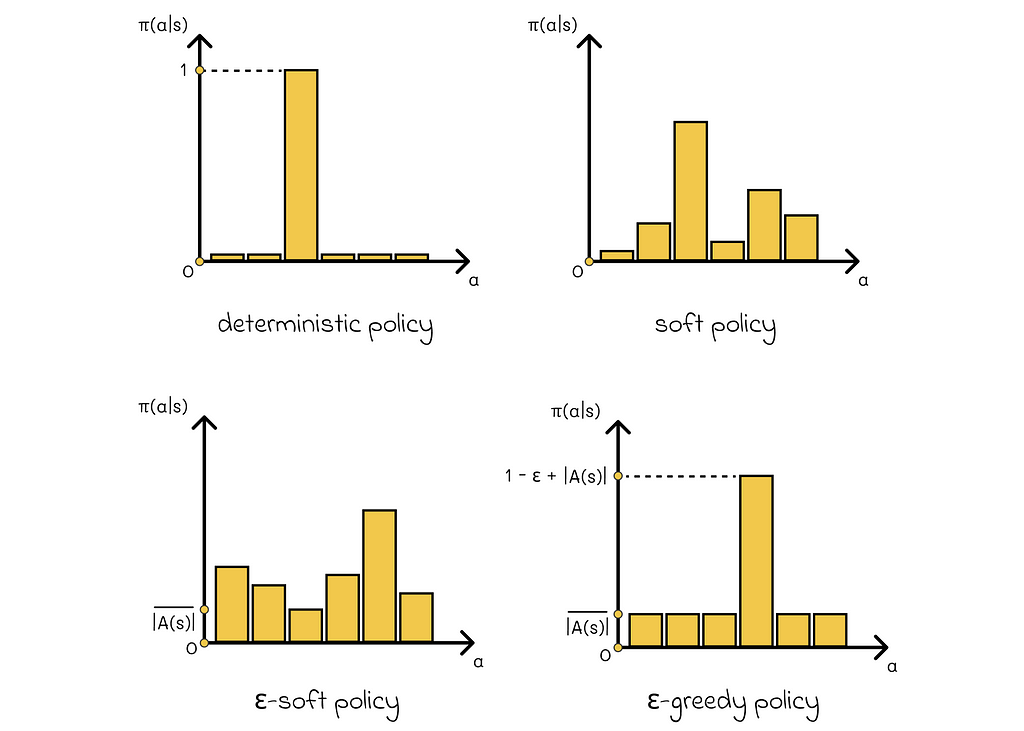
By the definition of the ε-greedy policy, any action can be chosen equiprobably with the probability p = ε / |A(s)|. The rest of the probability, which is 1 — ε, is added to the action with the maximal return, thus its total probability is equal to p = 1 — ε + ε / |A(s)|.
The good news about ε-greedy policies is that they can be integrated into the policy improvement algorithm! According to the theory, GPI does not require the updated policy to be strictly greedy with respect to a value function. Instead, it can be simply moved towards the greedy policy. In particular, if the current policy is ε-soft, then any ε-greedy policy updated with respect to the V- or Q-function is guaranteed to be better than or equal to π.
Monte Carlo control
The search for the optimal policy in MC methods proceeds in the same way, as we discussed in the previous article for model-based algorithms. We start with the initialization of an arbitrary policy π and then policy evaluation and policy improvement steps alternate with each other.
The term “control” refers to the process of finding an optimal policy.

- The Q-function is computed by sampling many episodes and averaging the returns.
- Policy improvement is done by making the policy greedy (or ε-greedy) with respect to the current value function.

In theory, we would have to run an infinite number of episodes to get exact estimations of Q-functions. In practice, it is not required to do so, and we can even run only a single iteration of policy evaluation for every policy improvement step.
Another possible option is to update the Q-function and policy by using only single episodes. After the end of every episode, the calculated returns are used to evaluate the policy, and the policy is updated only for the states that were visited during the episode.
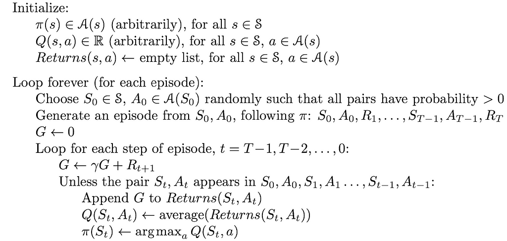
In the provided version of the exploring starts algorithm, all the returns for every pair (state, action) are taken into account, despite the fact that different policies were used to obtain them.
The algorithm version utilizing ε-greedy policies is exactly the same as the previous one, except for these small changes:
- π is initialized as an arbitrary ε-soft policy;
- the whole trajectory including the starting pair (S₀, A₀) is chosen according to the policy π;
- during update, the policy π always stays ε-greedy:

Example
By understanding how Monte Carlo control works, we are now all set to find optimal policies. Let us return to the blackjack example from the previous article, but this time we will look an optimal policy and its corresponding Q-function. Based on this example, we will make several useful observations.
Q-function
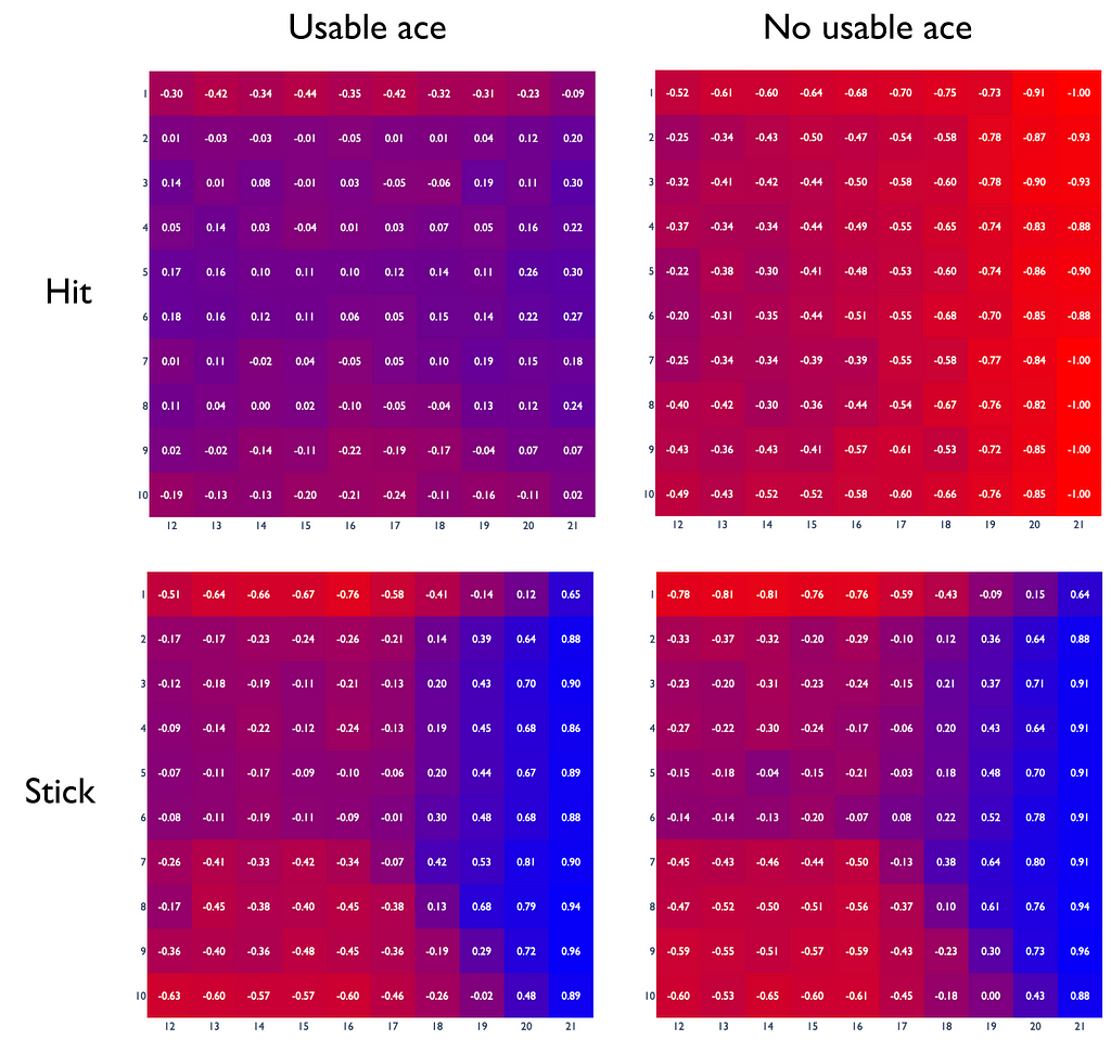
The constructed plot shows an example of the Q-function under an optimal policy. In reality, it might differ considerably from the real Q-function.
Let us take the q-value equal to -0.88 for the case when the player decides to hit having 21 points without a usable ace when the dealer has 6 points. It is obvious that the player will always lose in this situation. So why is the q-value not equal to -1 in this case? Here are the main two reasons:
- In the beginning of training, the algorithm does not know well which actions are better for certain states and picks them almost randomly. It might turn out that at some point, the difference of q-values between two actions becomes considerable. Therefore, during the policy improvement step, the algorithm will always greedily choose the action with the maximal reward. As a result, other actions with lower returns will never be sampled again and their true q-values will not be calculated adequately. If we look at the same state with the only difference of the dealer having 7 points, then the q-value is equal to -1 which is actually true. So as we can see, the algorithm converges differently for similar states due to its stochastic nature.
- We have set the α to 0.005 (explained in the section “Constant-α MC” below) which means that the algorithm needs some time to converge to the right answer. If we used more than 5 ⋅ 10⁶ iterations or used another value for α, than the estimated value could have been a little closer to -1.
Optimal policy
To directly obtain the optimal policy from the constructed Q-function, we only need compare returns for hit and stick actions in the same states and choose the actions whose q-values are greater.
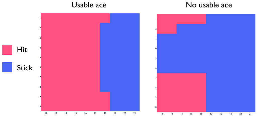
It turns out that the obtained blackjack policy is very close to the real optimal strategy. This fact indicates that we have chosen good hyperparameter values for ε and α. For every problem, their optimal values differ and should be chosen appropriately.
On-policy & off-policy methods
Consider a reinforcement learning algorithm that generates trajectory samples of an agent to estimate its Q-function under a given policy. Since some of the states are very rare, the algorithm explicitly samples them more often than they occur naturally (with explosing starts, for example). Is there anything wrong with this approach?
Indeed, the way the samples are obtained will affect the estimation of the value function and, as a consequence, the policy as well. As a result, we obtain the optimal policy that works perfectly under the assumption that the sampled data represents the real state distribution. However, this assumption is false: the real data has a different distribution.
The methods that do not take into account this aspect using differently sampled data to find the policy are called on-policy methods. The MC implementation we saw before is an example of an on-policy method.
On the other hand, there are algorithms that consider the data distribution problem. One of the possible solutions is to use two policies:
- the behaviour policy is used to generate sampled data.
- the target policy is learned and used to find the agent’s optimal strategy.
The algorithms using both behaviour and target policies are called off-policy methods. In practice, they are more sophisticated and more difficult to converge compared to on-policy methods but, at the same time, they lead to more precise solutions.
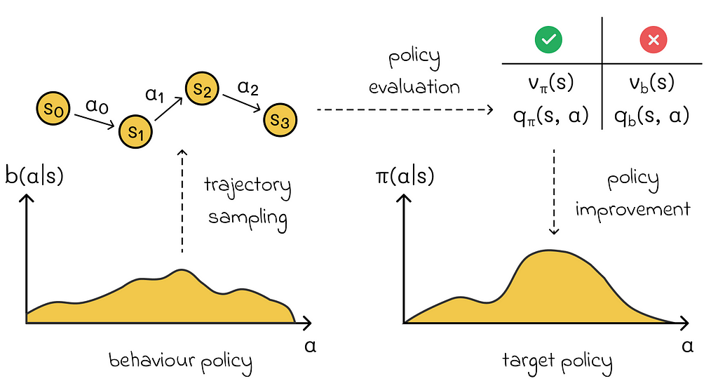
To be able to estimate the policy b through π, it is necessary to guarantee the coverage criteria. It states that π(a | s) > 0 implies b(a | s) > 0 for all a ∈ A and s ∈ S. In other words, for every possible action under policy π, there must be a non zero probability to observe that action in policy b. Otherwise, it would be impossible to estimate that action.
Now the question is how we can estimate the target policy if we use another behaviour policy to sample data? Here is where importance sampling comes into play, which is used in almost all off-policy methods.
Importance sampling
It is common in machine learning algorithms to calculate expected values. However, sometimes it can be hard and special techniques need to be used.
Motivation
Let us imagine that we have a data distribution over f(x) (where x is a multidimensional vector). We will denote by p(x) its probability density function.
We would like to find its expected value. By the integral definition, we can write:

Suppose that for some reasons it is problematic to calculate this expression. Indeed, calculating the exact integral value can be complex, especially when x contains a lot of dimensions. In some cases, sampling from the p distribution can be even impossible.
As we have already learned, MC methods allow to approximate expected values through averages:

Idea
The idea of importance sampling is to estimate the expected value of one variable (the target policy) through the distribution of another variable (the behaviour policy). We can denote another distribution as q. By using simple mathematical logic, let us derive the formula of expected value of p through q:

As a result, we can rewrite the last expression in the form of partial sums and use it for computing the original expected value.

What is fantastic about this result is that now values of x are sampled from the new distribution. If sampling from q is faster than p, then we get a significant boost to estimation efficiency.
Application
The last derived formula fits perfectly for off-policy methods! To make things more clear, let us understand its every individual component:
- Eₚ[f(x)] is the average return G under the target policy π we would like to ultimately estimate for a given state s.
- x corresponds to a single state s whose return we want to estimate; xᵢ is one out of N trajectories (observations) that passes through the state s.
- f(xᵢ) is the return G for state s.
- p(xᵢ) is the probability of getting the return G under the policy π.
- q(xᵢ) is the probability of getting the return G under the policy b.
Since the sampled data is obtained only via the policy b, in the formula notation, we cannot use x ~ p(x) (we only can do x ~ q(x)). That is why it makes sense to use importance sampling.
However, to apply the importance sampling to MC methods, we need to slightly modify the last formula.
- Recall that our goal is to calculate the Q-function under the policy π.

2. In MC methods, we estimate the Q-function under the policy b instead.

3. We use the importance sampling formula to estimate the Q-function under the policy π through the policy b.

4. We have to calculate probabilities of obtaining the reward G given the current state s and the agent’s next action a. Let us denote by t the starting moment of time when the agent is initially in the state s. T is the final timestamp when the current episode ends.

Then the desired probability can be expressed as the probability that the agent has the trajectory from sₜ to the terminal state in this episode. This probability can be written as the sequential product of probabilities of the agent taking a certain action leading it to the next state in the trajectory under a given policy (π or b) and transition probabilities p.

5. Despite not having knowledge of transition probabilities, we do not need them. Since we have to perform a division of p(Gₜ) under π over p(Gₜ) under b, transition probabilities present in both numerator and denominator will go away.

The resulting ratio ρ is called the importance-sampling ratio.
6. The computed ratio is plugged into the original formula to obtain the final estimation of the Q-function under the policy π.

If we needed to calculate the V-function instead, the result would be analogous:

The blackjack implementation we saw earlier is an on-policy algorithm, since the same policy was used during data sampling and policy improvement.
Incremental implementation
Another thing we can do to improve the MC implementation it to use the incremental implementation. In the given pseudocode above, we have to regularly recompute average values of state-action values. Storing returns for a given pair (S, A) in the form of an array and using it to recalculate the avreage when a new return value is added to the array is inefficient.
What we can do instead is to write the average formula in the recursive form:
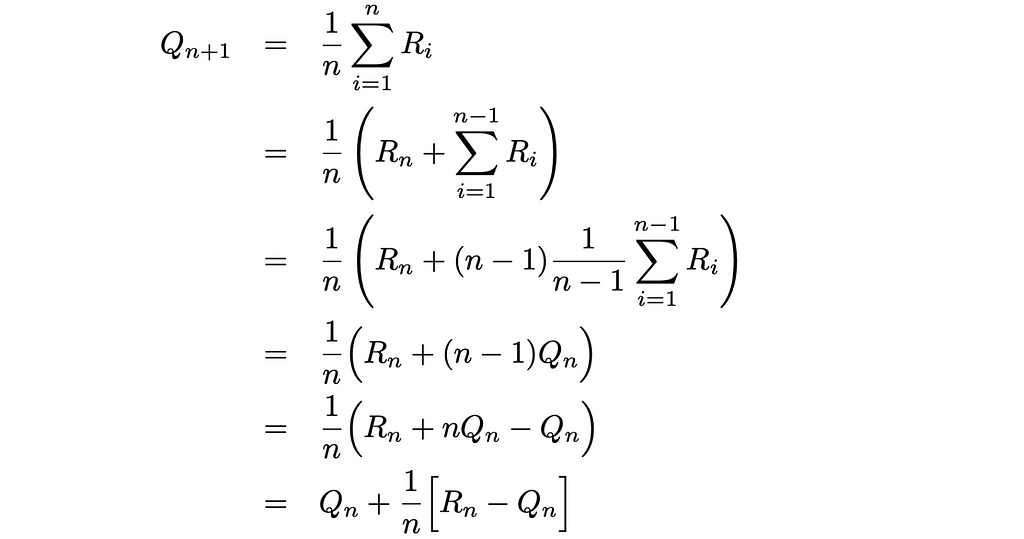
The obtained formula gives us an opportunity to update the current average as the function of the previous average value and a new return. By using this formula, our computations at every iteration require constant O(1) time instead of linear O(n) pass through an array. Moreover, we do not need to store the array anymore.
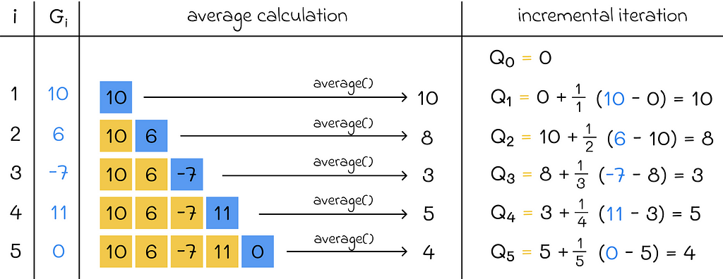
The incremental implementation is also used in many other algorithms that regularly recalculate average as new data becomes available.
Constant-α MC
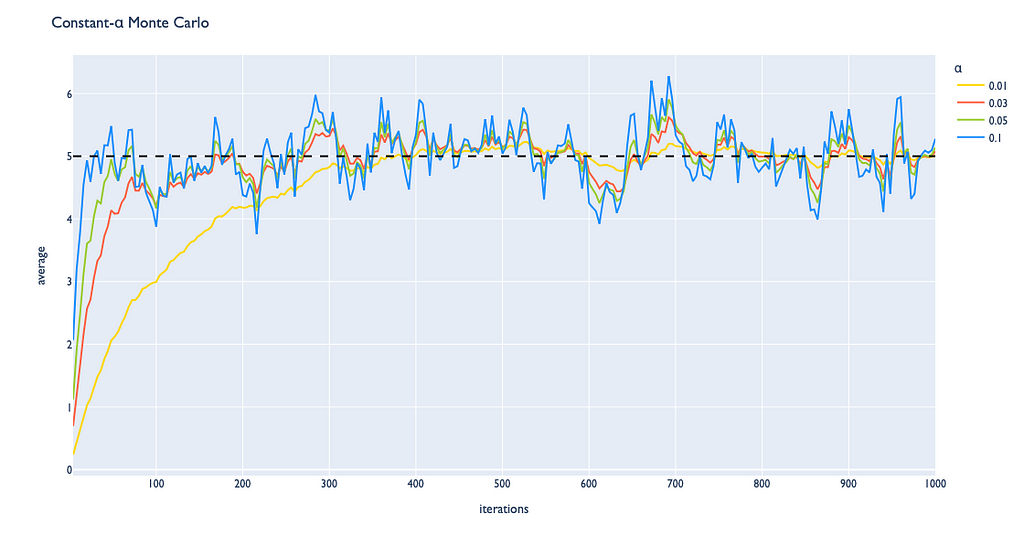
If we observe the update rule above, we can notice that the term 1 / n is a constant. We can generalize the incremental implementation by introducing the α parameter that replaces 1 / n which can be customly set to a positive value between 0 and 1.

With the α parameter, we can regulate the impact the next observed value makes on previous values. This adjustment also affects the convergence process:
- the smaller values of α make the algorithm converge slower to the true answer but lead to lower variance once estimated averages are located near the true average;
- the greater values of α make the algorithm converge faster to the true answer but lead to higher variance once estimated averages are located near the true average.
Conclusion
Finally, we have learned the difference between on-policy and off-policy approaches. While off-policy methods are harder to adjust appropriately in general, they provide better strategies. The importance sampling that was taken as an example for adjusting values of the target policy is one of the crucial techniques in reinforcement learning that is used in the majority of off-policy methods.
Resources
All images unless otherwise noted are by the author.
Reinforcement Learning, Part 4: Monte Carlo Control was originally published in Towards Data Science on Medium, where people are continuing the conversation by highlighting and responding to this story.


